SQL Window Functions are powerful tools that allow users to perform calculations across a set of table rows related to the current row.
Table of Contents
What is a Window Function?
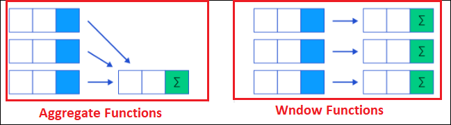
A window function performs a calculation across a set of table rows that are somehow related to the current row. This set of rows is referred to as the “window” and is defined using the OVER clause. Window functions are versatile and can be used for a wide range of analytical tasks.
Unlike aggregate functions, which return a single result for a group of rows, window functions can return multiple rows for each partition. This makes them incredibly useful for running totals, moving averages, and rank calculations.
Syntax
The general syntax for a window function is:
<function_name>(<expression>) OVER (
    [PARTITION BY <expression>]
    [ORDER BY <expression>]
    [ROWS/RANGE BETWEEN <start> AND <end>]
)- <function_name>: The window function to be used (e.g., ROW_NUMBER, RANK, SUM, AVG).
- <expression>: The column or expression to be used in the function.
- PARTITION BY: Divides the result set into partitions to which the window function is applied.
- ORDER BY: Defines the order of the rows within each partition.
- ROWS/RANGE BETWEEN: Specifies the window frame for the function.
Common Window Functions

Sample Data to practice with
CREATE TABLE employees (
    employee_id INT PRIMARY KEY,
    first_name VARCHAR(50),
    last_name VARCHAR(50),
    department_id INT,
    salary INT,
    hire_date DATE
);


INSERT INTO employees (employee_id, first_name, last_name, department_id, salary, hire_date) VALUES
(1, 'John', 'Doe', 101, 70000, '2018-04-12'),
(2, 'Jane', 'Smith', 101, 85000, '2017-03-09'),
(3, 'Alice', 'Johnson', 102, 60000, '2020-06-01'),
(4, 'Bob', 'Lee', 101, 85000, '2021-11-15'),
(5, 'Charlie', 'Brown', 103, 95000, '2016-07-23'),
(6, 'Eva', 'Green', 102, 67000, '2019-08-11'),
(7, 'David', 'Clark', 103, 95000, '2015-05-30'),
(8, 'Fiona', 'White', 101, 72000, '2020-01-10'),
(9, 'George', 'Black', 102, 60000, '2022-02-22'),
(10, 'Hannah', 'Scott', 103, 90000, '2018-12-03');
Sample Table
| employee_id | first_name | last_name | department_id | salary | hire_date |
|---|---|---|---|---|---|
| 1 | John | Doe | 101 | 70000 | 2018-04-12 |
| 2 | Jane | Smith | 101 | 85000 | 2017-03-09 |
| 3 | Alice | Johnson | 102 | 60000 | 2020-06-01 |
| 4 | Bob | Lee | 101 | 85000 | 2021-11-15 |
| 5 | Charlie | Brown | 103 | 95000 | 2016-07-23 |
| 6 | Eva | Green | 102 | 67000 | 2019-08-11 |
| 7 | David | Clark | 103 | 95000 | 2015-05-30 |
| 8 | Fiona | White | 101 | 72000 | 2020-01-10 |
| 9 | George | Black | 102 | 60000 | 2022-02-22 |
| 10 | Hannah | Scott | 103 | 90000 | 2018-12-03 |
ROW_NUMBER()
The ROW_NUMBER function assigns a unique sequential integer to rows within a partition of a result set, starting at 1 for the first row in each partition.
SELECT employee_id,first_name, last_name, department_id, salary, ROW_NUMBER() OVER
(PARTITION BY department_id ORDER BY salary DESC) AS row_num FROM employees;
Result:
| employee_id | first_name | last_name | department_id | salary | row_num |
|---|---|---|---|---|---|
| 4 | Bob | Lee | 101 | 85000 | 1 |
| 2 | Jane | Smith | 101 | 85000 | 2 |
| 8 | Fiona | White | 101 | 72000 | 3 |
| 1 | John | Doe | 101 | 70000 | 4 |
| 6 | Eva | Green | 102 | 67000 | 1 |
| 9 | George | Black | 102 | 60000 | 2 |
| 3 | Alice | Johnson | 102 | 60000 | 3 |
| 5 | Charlie | Brown | 103 | 95000 | 1 |
| 7 | David | Clark | 103 | 95000 | 2 |
| 10 | Hannah | Scott | 103 | 90000 | 3 |
RANK() and DENSE_RANK()
The RANK function assigns a rank to each row within a partition, with gaps in the ranking values when there are ties. DENSE_RANK assigns ranks without gaps.
SELECT employee_id, first_name, last_name, department_id, salary, RANK() OVER (PARTITION BY department_id ORDER BY salary DESC) AS rank, DENSE_RANK() OVER (PARTITION BY department_id ORDER BY salary DESC) AS dense_rank FROM employees;Result:
| employee_id | first_name | last_name | department_id | salary | rank | dense_rank |
|---|---|---|---|---|---|---|
| 4 | Bob | Lee | 101 | 85000 | 1 | 1 |
| 2 | Jane | Smith | 101 | 85000 | 1 | 1 |
| 8 | Fiona | White | 101 | 72000 | 3 | 2 |
| 1 | John | Doe | 101 | 70000 | 4 | 3 |
| 6 | Eva | Green | 102 | 67000 | 1 | 1 |
| 3 | Alice | Johnson | 102 | 60000 | 2 | 2 |
| 9 | George | Black | 102 | 60000 | 2 | 2 |
| 7 | David | Clark | 103 | 95000 | 1 | 1 |
| 5 | Charlie | Brown | 103 | 95000 | 1 | 1 |
| 10 | Hannah | Scott | 103 | 90000 | 3 | 2 |
Explanation:
- RANK() leaves gaps when there are ties.
- DENSE_RANK() gives the same rank to ties but does not skip ranks.
For example:
- In department 101, both Jane and Bob earn 85000 → RANK = 1, next gets RANK = 3.
- But DENSE_RANK = 1, and next gets DENSE_RANK = 2.
How Ties Are Determined:
A “tie” happens when two or more rows have identical values in the ORDER BY column(s) within their partition.
So here:
- Rows are first partitioned by department_id, so employees are grouped by department.
- Then within each department group, rows are ordered by salary DESC.
- If multiple employees have the same salary in the same department, they are considered a tie.
SQL RANK() versus ROW_NUMBER()
- RANK and DENSE_RANK are deterministic, all rows with the same value for both the ordering and partitioning columns will end up with an equal result, whereas ROW_NUMBER will arbitrarily (non-deterministically) assign an incrementing result to the tied
- ROW_NUMBER: Returns a unique number for each row starting with 1. For rows that have duplicate values, numbers are arbitrarily assigned.
- Rank: Assigns a unique number for each row starting with 1, except for rows that have duplicate values, in which case the same ranking is assigned and a gap appears in the sequence for each duplicate ranking.
LAG() and LEAD()
The LAG function provides access to a row at a specified physical offset before the current row within the result set. LEAD does the same but for the row after the current row.
LAG() Function
LAG() provides access to a previous row’s value in the result set without using self-joins.
Syntax:
LAG(column_name, offset, default_value) OVER (PARTITION BY … ORDER BY …)- column_name: The column you want to look back on.
- offset: How many rows back you want to go (default is 1).
- default_value: What to return if there’s no previous row (default is NULL).
Use case:
- Compare each employee’s salary with the one ranked before them (e.g., to find salary differences).
LEAD() Function
LEAD() returns the value of a subsequent (next) row in the result set.
Syntax:
LEAD(column_name, offset, default_value) OVER (PARTITION BY … ORDER BY …)Use case:
- Compare each employee’s value with the next row (e.g., find the next salary in the department).
SELECT employee_id,first_name,last_name,department_id,salary,
  LAG(salary, 1) OVER (PARTITION BY department_id ORDER BY salary DESC) AS previous_salary,
  LEAD(salary, 1) OVER (PARTITION BY department_id ORDER BY salary DESC) AS next_salary
FROM employees;Result:
| employee_id | first_name | last_name | department_id | salary | previous_salary | next_salary |
|---|---|---|---|---|---|---|
| 2 | Jane | Smith | 101 | 85000 | NULL | 85000 |
| 4 | Bob | Lee | 101 | 85000 | 85000 | 72000 |
| 8 | Fiona | White | 101 | 72000 | 85000 | 70000 |
| 1 | John | Doe | 101 | 70000 | 72000 | NULL |
| 6 | Eva | Green | 102 | 67000 | NULL | 60000 |
| 3 | Alice | Johnson | 102 | 60000 | 67000 | 60000 |
| 9 | George | Black | 102 | 60000 | 60000 | NULL |
| 5 | Charlie | Brown | 103 | 95000 | NULL | 95000 |
| 7 | David | Clark | 103 | 95000 | 95000 | 90000 |
| 10 | Hannah | Scott | 103 | 90000 | 95000 | NULL |
Explanation:
- LAG(salary, 1) gives the salary of the previous row in the department (by descending salary).
- LEAD(salary, 1) gives the salary of the next row in the department (by descending salary).
- NULL appears when there’s no previous or next row in that group.
Application
Example 1: Trend Analysis (e.g., Salary Changes, Stock Prices)
- Use: Compare current value with previous or next row.
- Example: Check if an employee’s salary increased or decreased over time.
Data set
CREATE TABLE employee_salaries (
    employee_id INT,
    salary INT,
    effective_date DATE
);

INSERT INTO employee_salaries (employee_id, salary, effective_date) VALUES
(1, 60000, '2019-01-01'),
(1, 65000, '2020-01-01'),
(1, 70000, '2021-01-01'),
(2, 80000, '2019-01-01'),
(2, 85000, '2021-01-01'),
(3, 50000, '2020-06-01'),
(3, 55000, '2021-06-01'),
(3, 60000, '2022-06-01');
Query
SELECT
  employee_id,
  effective_date,
  salary,
  LAG(salary) OVER (PARTITION BY employee_id ORDER BY effective_date) AS previous_salary,
  salary - LAG(salary) OVER (PARTITION BY employee_id ORDER BY effective_date) AS salary_change
FROM employee_salaries;
Output
| employee_id | effective_date | salary | previous_salary | salary_change |
|---|---|---|---|---|
| 1 | 2019-01-01 | 60000 | NULL | NULL |
| 1 | 2020-01-01 | 65000 | 60000 | 5000 |
| 1 | 2021-01-01 | 70000 | 65000 | 5000 |
| 2 | 2019-01-01 | 80000 | NULL | NULL |
| 2 | 2021-01-01 | 85000 | 80000 | 5000 |
| 3 | 2020-06-01 | 50000 | NULL | NULL |
| 3 | 2021-06-01 | 55000 | 50000 | 5000 |
| 3 | 2022-06-01 | 60000 | 55000 | 5000 |
Example 2: Detecting Gaps or Anomalies
- Use: Identify missing records or inconsistencies.
- Example: In a time series, use LAG() to find skipped dates or missing transactions.
CREATE TABLE user_logins (
  user_id INT,
  login_date DATE
);


INSERT INTO user_logins (user_id, login_date) VALUES
(1, '2024-01-01'),
(1, '2024-01-02'),
(1, '2024-01-04'),  -- gap: missing 2024-01-03
(1, '2024-01-05'),
(1, '2024-01-08');  -- gap: missing 2024-01-06, 2024-01-07
Query
SELECT
  user_id,
  login_date,
  LAG(login_date) OVER (PARTITION BY user_id ORDER BY login_date) AS previous_login,
  DATEDIFF(login_date, LAG(login_date) OVER (PARTITION BY user_id ORDER BY login_date)) AS gap
FROM user_logins;Output
| user_id | login_date | previous_login | gap |
|---|---|---|---|
| 1 | 2024-01-01 | NULL | NULL |
| 1 | 2024-01-02 | 2024-01-01 | 1 |
| 1 | 2024-01-04 | 2024-01-02 | 2 ← gap (2024-01-03 missing) |
| 1 | 2024-01-05 | 2024-01-04 | 1 |
| 1 | 2024-01-08 | 2024-01-05 | 3 ← gap (2024-01-06 & 07 missing) |
Example 3: Customer Retention / Churn Analysis
- Use: Find the time between customer interactions (purchases, logins, etc.).
- Example: Use LAG() to calculate days since last purchase.
Data sample
CREATE TABLE purchases (
    customer_id INT,
    purchase_date DATE
);
INSERT INTO purchases (customer_id, purchase_date) VALUES
(1, '2023-01-05'),
(1, '2023-02-15'),
(1, '2023-03-22'),
(2, '2023-01-10'),
(2, '2023-06-25'),
(3, '2023-03-05');
Query
SELECT
  customer_id,
  purchase_date,
  LAG(purchase_date) OVER (
    PARTITION BY customer_id
    ORDER BY purchase_date
  ) AS previous_purchase,
  DATEDIFF(
    purchase_date,
    LAG(purchase_date) OVER (
      PARTITION BY customer_id
      ORDER BY purchase_date
    )
  ) AS days_since_last_purchase
FROM purchases;Output
| customer_id | purchase_date | previous_purchase | days_since_last_purchase |
|---|---|---|---|
| 1 | 2023-01-05 | NULL | NULL |
| 1 | 2023-02-15 | 2023-01-05 | 41 |
| 1 | 2023-03-22 | 2023-02-15 | 35 |
| 2 | 2023-01-10 | NULL | NULL |
| 2 | 2023-06-25 | 2023-01-10 | 166 |
| 3 | 2023-03-05 | NULL | NULL |
Moving Average
A moving average calculates the average of a set of values over a sliding window of rows. It’s often used to smooth out short-term fluctuations and highlight trends.
Sample data
CREATE TABLE daily_sales (
    region VARCHAR(20),
    sale_date DATE,
    sales_amount INT
);

INSERT INTO daily_sales (region, sale_date, sales_amount) VALUES
('East', '2023-05-01', 100),
('East', '2023-05-02', 120),
('East', '2023-05-03', 90),
('East', '2023-05-04', 130),
('East', '2023-05-05', 110),
('West', '2023-05-01', 90),
('West', '2023-05-02', 130),
('West', '2023-05-03', 115),
('West', '2023-05-04', 140),
('West', '2023-05-05', 120);
Query
SELECT
  region,
  sale_date,
  sales_amount,
  AVG(sales_amount) OVER (
    PARTITION BY region
    ORDER BY sale_date
    ROWS BETWEEN 2 PRECEDING AND CURRENT ROW
  ) AS moving_avg_3_days
FROM daily_sales;
Output
| sale_date | sales_amount | moving_avg_3_days |
|---|---|---|
| 2023-05-01 | 100 | 100.0 |
| 2023-05-02 | 120 | 110.0 |
| 2023-05-03 | 90 | 103.3 |
| 2023-05-04 | 130 | 113.3 |
| 2023-05-05 | 110 | 110.0 |
Cumulative Distribution
Calculating the cumulative distribution of salaries within each department.
SELECT employee_id, first_name, last_name, department_id, salary, CUME_DIST() OVER (PARTITION BY department_id ORDER BY salary) AS cum_dist FROM employees;Result:
| employee_id | first_name | last_name | department_id | salary | cum_dist |
|---|---|---|---|---|---|
| 1 | John | Doe | 101 | 70000 | 0.2500000000 |
| 8 | Fiona | White | 101 | 72000 | 0.5000000000 |
| 4 | Bob | Lee | 101 | 85000 | 1.0000000000 |
| 2 | Jane | Smith | 101 | 85000 | 1.0000000000 |
| 9 | George | Black | 102 | 60000 | 0.6666666667 |
| 3 | Alice | Johnson | 102 | 60000 | 0.6666666667 |
| 6 | Eva | Green | 102 | 67000 | 1.0000000000 |
| 10 | Hannah | Scott | 103 | 90000 | 0.3333333333 |
| 5 | Charlie | Brown | 103 | 95000 | 1.0000000000 |
| 7 | David | Clark | 103 | 95000 | 1.0000000000 |
Explanation
Assume department 101 has 4 employees with salaries:
- 70000
- 72000
- 85000
- 85000
CUME_DIST() for each salary:
| salary | CUME_DIST() | Explanation |
|---|---|---|
| 70000 | 1/4 = 0.25 | One out of four salaries ≤ 70000 |
| 72000 | 2/4 = 0.50 | Two out of four salaries ≤ 72000 |
| 85000 | 4/4 = 1.00 | Four out of four salaries ≤ 85000 (both tied rows) |
What the output tells you:
- The cum_dist value is a percentile rank of each employee’s salary within their department.
- A value close to 0 means the employee’s salary is among the lowest in their department.
- A value close to 1 means the employee’s salary is among the highest.
Why is this useful?
- You can understand how an employee’s salary compares to peers in the same department.
- Useful for salary benchmarking, compensation analysis, or percentile-based reports.
Common Window functions
PERCENT_RANK()
Calculates the relative rank of a row as a percentage between 0 and 1.
Formula:
Percent rank = rank−1/total_rows−1- Use case: To get percentile rank of a value.
- Example: Employees’ salaries percentile within a department.
FIRST_VALUE()
Returns the first value in the window frame. To get the earliest or minimum value according to ordering.
Example:
FIRST_VALUE(salary) OVER (PARTITION BY department_id ORDER BY hire_date)LAST_VALUE()
Returns the last value in the window frame.
Note: Be careful, default frame includes rows up to current row; to get last overall value, frame specification might be needed.
Use case: Get the latest or maximum value in a partition.
Example:
LAST_VALUE(salary) OVER (PARTITION BY department_id ORDER BY hire_date ROWS BETWEEN UNBOUNDED PRECEDING AND UNBOUNDED FOLLOWING)LAST_VALUE() — seems broken
FIRST_VALUE() — works fine
SELECT
  department_id,
  employee,
  salary,
  FIRST_VALUE(salary) OVER (
    PARTITION BY department_id
    ORDER BY salary
  ) AS first_sal
FROM employees;| department_id | employee | salary | first_sal |
|---|---|---|---|
| 10 | A | 1000 | 1000 |
| 10 | B | 2000 | 1000 |
| 10 | C | 3000 | 1000 |
| 20 | D | 1500 | 1500 |
| 20 | E | 2500 | 1500 |
- Works fine — because the frame always starts at the first row,
- so the “first value” never changes.
LAST_VALUE() — seems broken at first
SELECT
  department_id,
  employee,
  salary,
  LAST_VALUE(salary) OVER (
    PARTITION BY department_id
    ORDER BY salary
  ) AS last_sal
FROM employees;| department_id | employee | salary | last_sal |
|---|---|---|---|
| 10 | A | 1000 | 1000 ❌ |
| 10 | B | 2000 | 2000 ❌ |
| 10 | C | 3000 | 3000 ✅ |
| 20 | D | 1500 | 1500 ❌ |
| 20 | E | 2500 | 2500 ✅ |
Why wrong?
- rows 1–2 → last value = 2000
- not the true last (3000).
Because the default frame ends at the current row, so for row 2 it only sees:
Fixing LAST_VALUE()
To make LAST_VALUE() see the entire partition, expand the frame manually:
SELECT
  department_id,
  employee,
  salary,
  LAST_VALUE(salary) OVER (
    PARTITION BY department_id
    ORDER BY salary
    ROWS BETWEEN UNBOUNDED PRECEDING AND UNBOUNDED FOLLOWING
  ) AS last_sal
FROM employees;| department_id | employee | salary | last_sal |
|---|---|---|---|
| 10 | A | 1000 | 3000 ✅ |
| 10 | B | 2000 | 3000 ✅ |
| 10 | C | 3000 | 3000 ✅ |
| 20 | D | 1500 | 2500 ✅ |
| 20 | E | 2500 | 2500 ✅ |
Visual Frame Movement
| Row | Salary | Default Frame (UNBOUNDED PRECEDING → CURRENT ROW) | Expanded Frame (UNBOUNDED PRECEDING → UNBOUNDED FOLLOWING) |
|---|---|---|---|
| 1 | 1000 | [1000] | [1000,2000,3000] |
| 2 | 2000 | [1000,2000] | [1000,2000,3000] |
| 3 | 3000 | [1000,2000,3000] | [1000,2000,3000] |
Rule of Thumb
Whenever you use LAST_VALUE() or NTH_VALUE(), always specify the frame explicitly:
ROWS BETWEEN UNBOUNDED PRECEDING AND UNBOUNDED FOLLOWINGNTH_VALUE()
Returns the nth value in the window frame.
Use case: Get a specific value from the sorted partition.
Example:
NTH_VALUE(salary, 2) OVER (PARTITION BY department_id ORDER BY hire_date)
Aggregate functions as window functions
You can also use regular aggregates as window functions, like:
- SUM()
- AVG()
- MIN()
- MAX()
- COUNT()
Query
SUM(salary) OVER (PARTITION BY department_id ORDER BY hire_date ROWS BETWEEN UNBOUNDED PRECEDING AND CURRENT ROW)Calculates running total of salary within each department ordered by hire date.
Common use cases
- Ranking and Leaderboards
- Use: Show top performers, ranks by sales, scores, performance, etc.
- Functions: RANK(), DENSE_RANK(), ROW_NUMBER()
- Example: Top 3 earners per department.
- Running Totals / Cumulative Sums
- Cumulative sales over time per customer or region.
- Running balance in a bank account.
- Cumulative profit/loss in financial reports.
- Total number of signups up to each day.
- Tracking cumulative expenses in a budget.
- Inventory tracking (stock added vs. sold over time).
- User activity streaks (e.g., consecutive login days).
- Points accumulated in games or reward systems.
- Project progress tracking (e.g., tasks completed over time).
- Employee work hours logged over time.
- First / Last Value per Group : FIRST_VALUE(), LAST_VALUE()
- Get the earliest hire date or join date of employees in each department
- Find the first purchase date for each customer
- Retrieve the latest transaction or activity date per user
- Identify the initial or most recent status update in workflows
- Extract the opening or closing price of a stock per trading day or period
- De-duplication / Keeping Latest Entry :ROW_NUMBER() in a CTE
- Selecting the most recent record per user, customer, or entity (e.g., latest login, last purchase, newest update) to avoid duplicates and keep only the latest data entry.
De duplication
Way 1 With Window function
DELETE FROM employees
WHERE id IN (
  SELECT id
  FROM (
    SELECT id,
           ROW_NUMBER() OVER (PARTITION BY email ORDER BY id) AS rn
    FROM employees
  ) t
  WHERE rn > 1
);Explanation
DELETE FROM employees
WHERE id IN (
  SELECT id
  FROM (query_1) t
  WHERE rn > 1
);

or

DELETE FROM employees WHERE id IN (query_2);


query 1:
SELECT id, ROW_NUMBER() OVER (PARTITION BY email ORDER BY id) AS rn FROM employees

query 2:
SELECT id FROM (query_1) t WHERE rn > 1
Query 1: The OVER (PARTITION BY email ORDER BY id) splits the employees rows into groups by email.
Query 2:
- Get all id except the id where ROW_NUMBER is 1
- t is just an alias — it gives a name to the inner subquery result, so that the outer query can legally reference its columns (rn in this case).
- Without the alias t, the query will fail with an error like:”Every derived table must have its own alias”
Last step
- DELETE FROM employees WHERE id IN (query_2);
- Delete all except where ROW_NUMBER is 1
CTE form
WITH duplicates AS (
  SELECT id
  FROM (
    SELECT id,
           ROW_NUMBER() OVER (PARTITION BY email ORDER BY id) AS rn
    FROM employees
  ) t
  WHERE rn > 1
)


DELETE FROM employees WHERE id IN (SELECT id FROM duplicates);Explanation
Step 1
- Creates a CTE (Common Table Expression) named duplicates.
- For each user_id, it assigns a row number rn starting at 1 for the most recent event_date (because of ORDER BY event_date DESC).
- So for each user, the latest event gets rn = 1, the second latest rn = 2, and so on.
Step 2
- This part deletes rows from the original user_events table.
- It deletes rows where the user_id and event_date match any rows in duplicates where rn > 1 — i.e., all but the latest event for each user.
- So effectively, it keeps the latest entry (rn = 1) for each user and deletes the rest (duplicates or older entries).
Way 2 Without window function
DELETE FROM employees
WHERE id NOT IN (
  SELECT id FROM (
    SELECT MIN(id) AS id
    FROM employees
    GROUP BY email
  ) t
);Way 3: Join
DELETE e1
FROM employees e1
JOIN employees e2
  ON e1.email = e2.email
AND e1.id > e2.id;- Keeps the row with the smallest id for each email.
- Works on old and new MySQL versions.
- e1.id > e2.id → ensures that we only pick the newer (higher id) row for deletion.
- Replace email with your duplicate-defining column(s).
Example
| id | name | |
|---|---|---|
| 1 | John | john@gmail.com |
| 2 | Mary | mary@gmail.com |
| 3 | John | john@gmail.com |
| 4 | John | john@gmail.com |
Intermediate
e1.email = e2.email
| e1_id 1 | e1_name | e1_email | e2_id | e2_name | e2_email |
|---|---|---|---|---|---|
| 1 | John | john@gmail.com | 1 | John | john@gmail.com |
| 1 | John | john@gmail.com | 3 | John | john@gmail.com |
| 1 | John | john@gmail.com | 4 | John | john@gmail.com |
| 2 | Mary | mary@gmail.com | 2 | Mary | mary@gmail.com |
| 3 | John | john@gmail.com | 4 | John | john@gmail.com |
| 3 | John | john@gmail.com | 1 | John | john@gmail.com |
| 3 | John | john@gmail.com | 3 | John | john@gmail.com |
| 4 | John | john@gmail.com | 1 | John | john@gmail.com |
| 4 | John | john@gmail.com | 3 | John | john@gmail.com |
| 4 | John | john@gmail.com | 4 | John | john@gmail.com |
Candidate for deletion: e1.email = e2.email and e1.id > e2.id
| e1_id | e1_name | e1_email | e2_id | e2_name | e2_email |
|---|---|---|---|---|---|
| 3 | John | john@gmail.com | 1 | John | john@gmail.com |
| 4 | John | john@gmail.com | 1 | John | john@gmail.com |
| 4 | John | john@gmail.com | 3 | John | john@gmail.com |
Final Table
| id | name | |
|---|---|---|
| 1 | John | john@gmail.com |
| 2 | Mary | mary@gmail.com |
Conclusion
SQL Window Functions are incredibly powerful tools for performing complex calculations across a set of table rows related to the current row. By using the OVER clause, these functions can provide insights and analytics that are difficult to achieve with standard SQL queries. Understanding and leveraging these functions can greatly enhance your ability to perform data analysis and gain meaningful insights from your datasets.
Use the examples provided in this article to experiment with window functions and see how they can be applied to your specific use cases. With practice, you’ll be able to harness the full power of SQL Window Functions to perform advanced data analysis with ease.
2 thoughts on “Understanding SQL Window Functions: A Comprehensive Guide”